How to make a dynamic dependent dropdown list in Excel an easy way

adminMarch 11, 2023

0 60 6 minutes read

How to create dynamic changing drop-down lists in excel

YOU ARE READING: How to make a dynamic dependent dropdown list in Excel an easy way AT Vccidata_En

The tutorial shows how to create an Excel dropdown list dependent on another cell using new dynamic array functions.

Creating a simple dropdown list in Excel is easy . Creating a multi-level cascading drop-down menu has always been a challenge. The tutorial linked above describes four different approaches, each containing a crazy number of steps, a bunch of different formulas, and a handful of limitations regarding multi-word entries, empty cells, etc.

Reading: How to create dynamic changing drop-down lists in excel

That’s bad news . The good news is that these methods were designed for pre-dynamic versions of Excel. The introduction of dynamic arrays in Excel 365 changed everything! With new dynamic array functions, creating a multi-dependent dropdown list is a matter of minutes, if not seconds. No tricks, no caveats, no nonsense. Just quick, no-fuss, easy-to-understand solutions.

Create a dynamic dropdown list in Excel
Create a multi-dependent dropdown list
Create an expandable dropdown list without empty cells
Sort dropdown list alphabetically

How to create dynamic dropdown list in Excel

This Example demonstrates the general approach to creating a cascading drop-down list in Excel using the new dynamic array functions.

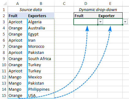
Suppose you have a list of fruits in column A and exporters in column B. There is an additional complication in that the fruit names are not grouped but scattered across the column. The goal is to put the unique fruit names in the first dropdown menu and depending on the user’s selection, display the relevant exporters in the second dropdown menu. Source data for a dependent drop-down list

To create a dynamic dependent drop-down list in Excel, run it from Steps:

1. Retrieving items for the main dropdown list

First we will extract all the different fruit names from column A. This can be done by using the UNIQUE function in its simplest form – first supply the fruit list argument (array) and omit the remaining optional arguments as their default values work fine for us:

= UNIQUE(A3:A15)

The formula goes to G3, and after pressing the Enter key, the results are automatically transferred to the next cells in the main drop-down list” />

2.Create the main drop-down list

To create your primary drop-down list, configure an Excel data validation rule like this:

Select a cell where you want the drop-down list to appear (D3 in our case).
On the Data tab, in the Data Tools group, click Data Validation.
In the “Data Validation” dialog box, do the following:
- Under Allow, select List.
- Give In the Source field, enter the reference to the overflow range that the UNIQUE formula outputs. To do this, type the hash tag right after the cell reference, like this: =$G$3#
  This is called a spill range reference, and this syntax refers to the entire range, no matter how much it spills or spills is shortened.
- Click OK to close the dialog box.

Your primary dropdown is ready! The first dropdown is done.

3. Get items for the dependent dropdown

To get items for the secondary dropdown, we filter the values in column B based on the value selected in the first dropdown. This can be done using another dynamic array function called FILTER:

=FILTER(B3:B15, A3:A15=D3)

Where B3:B15 is the source data for your dependent dropdown, A3:A15 is the source data for your main dropdown and D3 is the main dropdown cell.

To ensure the formula works correctly, you can enter a value in the first dropdown select -down list and observe the results returned by FILTER. Perfect! 🙂 Get items for dependent dropdown

4. Create the dependent dropdown

To create the second dropdown, configure the data validation criteria exactly as you did for the first dropdown in step 2. However, this time refer to the overflow area returned by the FILTER function : =$H$3# Configuring dependent drop-down list

That’s it! Your Excel dependent dropdown list is ready to use. One dependent dropdown list in Excel

How to create multiple dependent dropdown lists in Excel

In the previous example, we made a dropdown list dependent on another cell. But what if you need a multi-level hierarchy, i.e. a third drop-down menu depending on the second list, or even a fourth drop-down menu depending on the third list. Is that possible? Yes, you can set up any number of dependent lists (a reasonable number of course :).

For this example we have placed states/provinces in column C and now want to add a corresponding dropdown menu in G3: Source data for a multi-dependent dropdown list

Um To create a multi-dependent dropdown list in Excel, you need to do the following:

1 Set up the first dropdown L iste ein

The main dropdown list is created using exactly the same steps as in the previous example (see steps 1 and 2 above). The only difference is the overflow range reference that you enter in the source field.

This time the UNIQUE formula is in E8 and the main dropdown list will be in E3. So you select E3, click Data Validation and provide this reference: =$E$8# Setting up the first drop-down list

2. Configure the second drop-down menu

As you may have noticed, column B now contains multiple occurrences of the same exporters. But you only want unique names in your dropdown list, right? To omit all duplicate occurrences, wrap the UNIQUE function around your FILTER formula and enter this updated formula in F8:

=UNIQUE(FILTER(B3:B15, A3:A15=E3))

Where B3:B15 is the source data for the second dropdown, A3:A15 is the source data for the first dropdown, and E3 is the first dropdown cell.

After that, use the following Overflow area reference for the data validation criteria: =$F$8#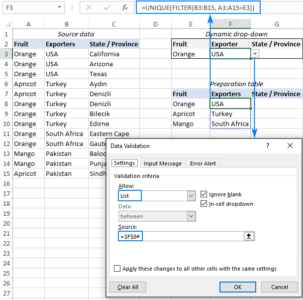 Configuring the second dropdown

3. Set up the third drop-down list

To collect the items for the third drop-down list, use the FILTER formula with multiple criteria. The first criterion checks the entire fruit list against the value selected in the 1st dropdown (A3:A15=E3), while the second criterion checks the list of exporters against the selection in the 2nd dropdown (B3:B15=F3). The full formula goes to G8:

=FILTER(C3:C15, (A3:A15=E3) * (B3:B15=F3))

If you add more dependent dropdowns (4th, 5th, etc.), column C most likely contains multiple occurrences of the same item. To prevent duplicates from entering the prepare table and consequently the 3rd drop-down list, nest the FILTER formula inside the UNIQUE function as we did in the previous step:

=UNIQUE (FILTER(C3:C15, ( A3:A15=E3) * (B3:B15=F3)))

The last thing you need to do is to create another data validation rule with this source reference: =$G$8# Set up third dropdown

Your multi-dependent dropdown list is ready to go!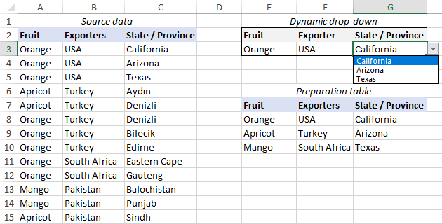 Dropdown list with multiple dependencies in Excel

How to create an expandable dropdown list in Excel

Once you’ve created a dropdown list, your first concern might be what happens when You add new elements to the source data. Does the dropdown list update automatically? If your original data is formatted as an Excel spreadsheet, yes, then a dynamic drop-down list discussed in the previous examples will auto-expand without your effort as Excel spreadsheets are inherently extensible.

If so, for some reason using an Excel spreadsheet is not an option, you can make your dropdown list expandable this way:

To new data automatically To include when adding them to the source list, add a few extra cells to the arrays referenced in your formulas.
To exclude empty cells , configure the formulas to ignore empty cells until they are filled.

Remember these two points and tweak the formulas in our data prep spreadsheet. The data validation rules do not require any adjustments at all.

Main dropdown formula

With the fruit names in A3:A15, we add 5 additional cells to the array to account for possible new ones entries. Also, we embed the FILTER function in UNIQUE to extract unique values with no spaces.

From this, the formula in G3 takes this form:

=UNIQUE(FILTER(A3:A20, A3:A20″”))

Formula for the dependent dropdown

The formula in G3 doesn’t need to be changed much – just add a few more cells to the arrays:

=FILTER(B3:B20, A3:A20 =D3)

The result is a fully dynamic expandable dependent dropdown: Create an expandable drop-down list in Excel

Sort drop-down list alphabetically

Would you like to arrange your drop-down list alphabetically without having to reorganize the source data sort by ? The new dynamic Excel has a special function for this too! In your data prep table, simply wrap the SORT function around your existing formulas.

The data validation rules are configured exactly as described in the previous examples.

To sort from A to Z

h3>

Since ascending sort order is the default option, you can simply nest your existing formulas in the array argument of SORT and omit any other optional arguments.

For the main dropdown (the formula in G3):

=SORT(UNIQUE(FILTER(A3:A20, A3:A20″”)))

For the dependent dropdown (the formula in H3):

=SORT(FILTER(B3:B20, A3:A20=D3))

Done! Both drop-down lists are sorted alphabetically from A to Z alphabetically” />

To sort from Z to A

To sort in descending order, you must use the 3rd argument (sort_order ) of the SORT function to -1.

For the main dropdown(the formula in G3):

=SORT(UNIQUE(FILTER( A3:A20, A3:A20″”)) , 1, -1)

For the dependent dropdown(the formula in H3):

=SORT(FILTER(B3:B20, A3:A20 =D3), 1, -1)

This will sort both the data in the preparation table and the items in the drop-down lists from Z to A sorted: Sort a dropdown list descending

How to create dynamic dropdown list in Excel with the help of new dynamic array functions Unlike the traditional methods, this approach works perfectly for single and multi-word items and takes care of all empty ones cells. Thanks for reading and we hope to see you on our blog next week!