Some time ago we started exploring the possibilities of Excel data validation and learned how to create a simple dropdown list in Excel based on a comma separated list, a range of cells or a named range.
Today we’re going to explore this feature in depth and learn how to create cascading dropdown lists that display choices depending on the value selected in the first dropdown. To put it another way, we’re creating an Excel data validation list based on the value of another list.
Reading: How to create multiple dependent drop down lists in excel
- Creating a multi-dependent drop-down list
- Cascading drop-down lists of items with multiple words
- Block changes in the primary drop-down list
- Create a dynamic dependent drop-down list
- Blank lines from the dynamic drop-down -Exclude menu
How to create multiple dependent dropdown lists in Excel
Creating a multilevel dependent dropdown list in Excel is easy. All you need are a few named ranges and the INDIRECT formula. This method works with all versions of Excel 365 – 2010 and earlier.
1. Enter the entries for the drop-down lists
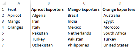
First enter the entries that you want to appear in the drop-down lists, each list in a separate column. For example, I am creating a cascading dropdown of fruit exporters and column A of my source sheet (fruit) contains the items of the first dropdown and three other columns list the items for the dependent dropdowns.
2. Creating Named Ranges
Now you need to create names for your master list and for each of the dependent lists. You can do this by either adding a new name in the Name Manager window (Formulas tab > Name Manager > New) or typing the name directly into the name field.
See How to define a name in Excel for detailed step-by-step instructions.
Notes:
- The items to appear in the first drop-down list must be one-word entries, e.g. Apricot, mango, oranges. If you have items that consist of two, three or more words, please see How to create a cascading drop-down menu with multi-word items.
- The names of the dependent lists must exactly match the Entry in matching main list. For example, the dependent list to be displayed when “Mango” is selected from the first drop-down list should be called Mango.
When you’re done, you can press Ctrl+F3 Open Open the Name Manager window and verify that all lists have correct names and references.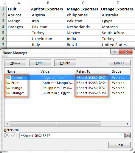
3. Create the first (main) drop-down list
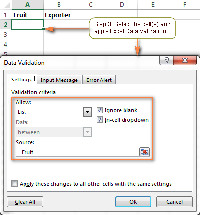
- In the same or another table, select one or more cells where you want your primary drop-down list to appear.
- Go to the Data tab, click Data Validation and set up a dropdown list based on a named range in the usual way by selecting List under Allow and select Enter the realm name in the Source field.
See Creating a drop-down list based on a named range for the detailed steps.
As a result, you will see a drop-down menu similar to the following in your worksheet:
4. Create the dependent dropdown list
Select one or more cells for your dependent dropdown menu and reapply the Excel data validation as described in the previous step. But this time, instead of naming the range, enter the following formula in the Source field:
=INDIRECT(A2)
Where A2 is the cell with your first (primary) drop-down List.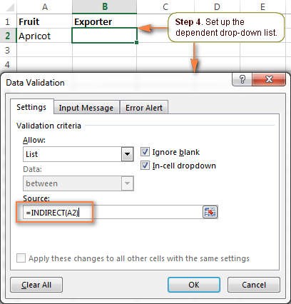
If cell A2 is currently empty, you will get the error message “The source is currently yielding an error. Do you want to continue?”
Be sure to click Yes and Once you have an entry from the first drop-down menu, you will see the corresponding entries in the second, dependent drop-down list.
5. Add a third dependent drop-down list (optional)
If needed, you can add a third cascading drop-down list that depends on either the selection in the second drop-down menu or the selection in the first two Dropdowns.
Set up third dropdown that depends on second list
You can create dropdown list of this type in the same way we just created a second dependent dropdown Menu. Just remember the two important things discussed above that are essential for your cascading dropdown lists to work correctly.
For example, if you want to display a list of regions in column C depending on which country is selected in column B, create a list of regions for each country and name them exactly after the country’s name how the country appears in the second drop-down lists. For example, a list of Indian regions should be named “India”, a list of Chinese regions should be named “China”, and so on.
Next, select a cell for the third drop-down menu (C2 in our case) and flip the Excel data validation with the following formula (B2 is the cell with the second dropdown menu containing a list of countries):
=INDIRECT(B2)
Now every time you select India under the country list in column B, you will have the following choices in the third drop-down menu:
Create a third dropdown depending on the first two lists
If you need to create a cascading dropdown that depends on the selections in both the first and second Drop-down depends on lists, then do the following:
- Create additional sets of named ranges and name them after the word combinations in your first two drop-down menus. For example, you have mango, oranges, etc. in the 1st list and India, Brazil, etc. in the 2nd list. Then create named ranges MangoIndia, MangoBrazil, OrangesIndia, OrangesBrazil etc. These names should not contain underscores or other additional characters.

- Apply Excel data validation with the INDIRECT REPLACEMENT formula, which concatenates the names of the entries in the first two columns and removes the spaces from the names. For example, in cell C2, the data validation formula would be:
=INDIRECT(SUBSTITUTE(A2&B2,” “,””))
See also: Postgres.app
Where A2 and B2 contain the first and second drop-down lists, respectively.
As a result, your 3rd drop-down list will display the regions corresponding to the fruit and country selected in the first 2 drop-down lists.

This is the easiest way to create cascading dropdown boxes in Excel. However, this method has a number of limitations.
Limitations of this approach:
- The items in your primary drop-down list must be one-word -Entries. Learn how to create cascading drop-down lists with multi-word items.
- This method will not work if the items in your main drop-down list contain characters that are not allowed in space names, such as . E.g. the hyphen (-), ampersand (&), etc. The solution is to create a dynamic cascading drop-down menu that does not have this limitation.
- Drop-down menus created this way will be not automatically updated d to change the named range references each time you add or remove items in the source lists. To overcome this limitation, try creating a dynamic cascading drop-down list.
Create cascading drop-down lists with multi-word entries
These of us The INDIRECT formulas used in the example above can only process one-word elements. For example, the formula =INDIRECT(A2) indirectly references cell A2 and displays the named range with exactly the same name as in the referenced cell. However, spaces are not allowed in Excel names, so this formula will not work with multi-word names.
The solution is to use the INDIRECT function in combination with SUBSTITUTE, as we did when creating a 3. Dropdown.
Suppose you have watermelon among the products. In this case, name a list of watermelon exporters with a word with no spaces – watermelon.
Then, for the second drop-down menu, apply Excel data validation with the following formula, which removes the spaces from the Names removed cell A2:
=INDIRECT(SUBSTITUTE(A2,” “,””))
Prevent changes in the primary drop-down list
Imagine the following scenario. Your user made the selection in all of the drop-down lists, then changed their mind, went back to the first list, and selected a different item. As a result, the 1st and 2nd choices are mismatched. To prevent this from happening, you may want to block any changes in the first drop-down list once a selection is made in the second list.
To do this, when creating the first drop-down menu, use a special formula that checks whether an item is selected in the second drop-down menu:
=IF(B2=”” , Fruit, INDIRECT(“FakeList”))
Where B2 contains the second drop-down menu, “Fruit” is the name of the list that appears in the first drop-down menu and “FakeList” is any fake Name that doesn’t exist.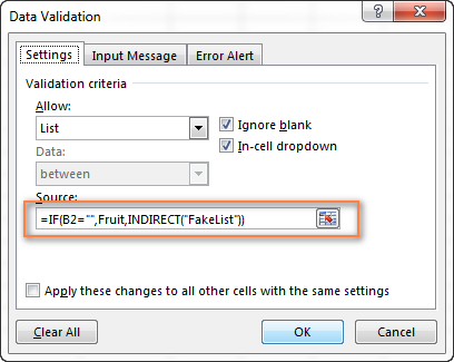
Now when an item is selected in the second drop-down list, no choices are available when the user clicks the arrow next to the first list.
Dynamic create cascading drop-down lists in Excel
The main advantage of a dynamic Excel-dependent drop-down list is that you can edit the source lists freely and your drop-down boxes can be a to be updated . Of course, creating dynamic dropdown menus requires a bit more time and more complex formulas, but I believe it’s a worthwhile investment as it’s really fun to work with such dropdown menus once set up.
As with almost everything in Excel, you can achieve the same result in different ways. Specifically, you can create a dynamic dropdown menu using a combination of OFFSET, INDIRECT, and COUNTA functions, or a more robust INDEX-MATCH formula. The latter is my preferred way as it offers numerous advantages, the most important of which are:
- You only need to create 3 named ranges, no matter how many items there are in the main and sub lists.
- Your lists can contain items with multiple words and any special characters.
- The number of entries can vary in each column.
- The sorting of the entries does not matter the order role.
- Finally, it’s very easy to maintain and change the source lists.
Okay, enough theory, let’s get down to practice.
1. Organize your source data in a table
As usual, you first need to write down all the choices for your drop-down lists in a worksheet. This time you need to save the source data in an Excel spreadsheet. To do this, after entering the data, select all entries and press Ctrl + T or click Insert Tab > Table. Then enter a name of your table in the Table Name field.
The most convenient and visual approach is to label the items for the first dropdown as table headers and the items for the dependent dropdown as table save data. The screenshot below illustrates the structure of my table named exporters_tbl – the fruit names are table headings and a list of exporting countries is added under the corresponding fruit name. 
2. Create Excel Names
Now that your source data is ready, it’s time to set up named references that will dynamically retrieve the correct list from your spreadsheet.
2.1. Add a name for the table header (main dropdown)
To create a new name that references the table header, select it and then either click Formulas > Name Management > New or press Ctrl + F3.
p>
Microsoft Excel uses the built-in table reference system to construct the pattern name table_name[#Headers].
Give it a descriptive and easy-to-remember name , e.g. fruit_list and click OK.
2.2. Create a name for the cell that will contain the first dropdown list
I know you don’t have a dropdown list yet 🙂 But you need to select the cell that will host your first dropdown list , and create a name for this cell now, because you need to include that name in the third name’s reference.
See also: How to insert a dynamic banner into header of website
For example, my first dropdown box is in cell B1 on sheet 2, so I create one Name it, something simple and self-explanatory like fruit: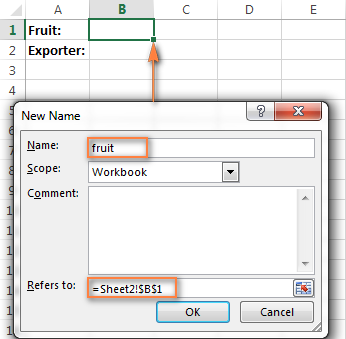
2.3. Create a name to retrieve the dependent menu items
Rather than setting up unique names for each of the dependent lists as we did in the previous example, we will create a named formula which is not associated with a specific cell or range of cells. Depending on the selection made in the first drop-down list, the correct list of entries for the second drop-down list will be retrieved. The main advantage of using this formula is that you don’t have to create new names when adding new entries to the first drop-down list – one named formula covers them all.
You create a new Excel Name with this formula:
=INDEX(exporters_tbl,,MATCH(fruit,fruit_list,0))
Where:
- exporters_tbl – the name of the table (created in step 1);
- Fruit – the name of the cell containing the first drop-down list (created in step 2.2);
- fruit_list – the name that refers to the table header (created in step 2.1).
I named it exporters_list, like you see screenshot below.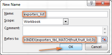
Well, you’ve already done most of the work! Before proceeding to the last step, it’s a good idea to open the Name Manager (Ctrl + F3) and check the names and references: 
3. Set up Excel data validation
This is actually the easiest part. With the two named formulas in place, set up data validation in the usual way (Data tab > Data Validation).
- For the first drop-down list in the Source field, enter = a fruit_list (the name created in step 2.1).
- For the dependent drop-down list, enter =exporters_list (the name created in step 2.3).
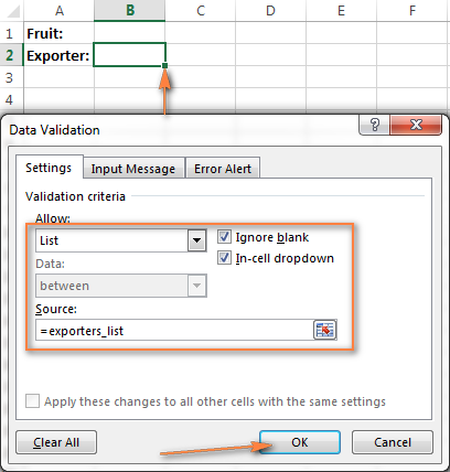
Done! Your dynamic cascading dropdown menu is ready and will be automatically updated to reflect the changes you made to the source spreadsheet.
Perfect in every other respect, this dynamic Excel dropdown menu has one downside – if the columns of your source table contain a different number of items, the empty rows will appear in your menu like this:
Exclude empty rows from dynamic cascading dropdown menu
If you want to delete all empty rows in your dropdown fields, you need to go one step further and improve them INDEX / MATCH formula used to create the dependent dynamic dropdown list.
The idea is to use 2 INDEX functions, the first one gets the top left cell and the second one gets the lower right cell returns the range or OFFSET function with nested INDEX and COUNTA. The detailed steps follow below:
1. Create two additional names
In order not to make the formula too cumbersome, first create some helper names with the following simple formulas:
- A name called col_num to refer to the selected column number:
=MATCH(fruit,fruit_list,0)
- A name called entire_col to refer to to reference the selected column (not the number of the column, but the entire column):
=INDEX(exporters_tbl,,col_num)
In the above formulas, exporters_tbl the name of your source table, fruit is the name of the cell that contains the first dropdown menu, and fruit_list is the name that references the table header.
2. Create the named reference for the dependent drop-down list
Next, use one of the following formulas to create a new name (let’s call it exporters_list2) to use with the dependent drop-down list :
=INDEX(exporters_tbl,1,col_num) : INDEX(exporters_tbl, COUNTA(entire_column), col_num)
=OFFSET(INDEX(exporters_tbl,1,col_num),0, 0,COUNTA(entire_column) )
3. Apply data validation
Finally, select the cell with the dependent drop-down menu and apply data validation by typing =exporters_list2 (the name created in the previous step) in the Source field.
The screenshot below shows the resulting dynamic dropdown menu in Excel with all blank lines gone!
How to create an Excel data validation list based on the values of another list. Please don’t hesitate to download our sample workbooks to see the cascading dropdowns in action. Thank you for reading!
Download exercise workbook
Cascading down example 1 – simple versionCascading down example 2 – extended version without spaces
See also: Create Web Pages by. Using HTML
You might also be interested in
- Custom data validation in Excel
- Easy way to add dynamic dependent dropdown menu in Excel 365
- Create dependent dropdown menu for multiple Rows
- How to create a drop down list with images in Excel
- How to create and use a data entry form in Excel
.