Reading time: 4 minutes
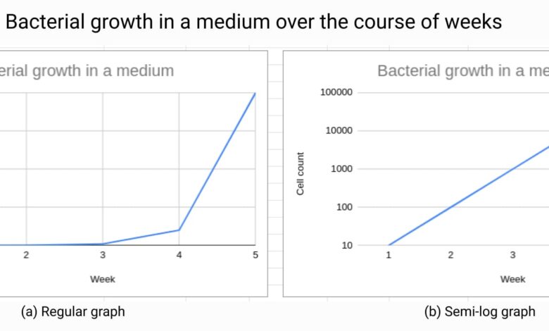
Over the past few years, you must have frequently come across graphs showing the spread of the coronavirus in various population groups – and how quickly it is spreading. They show exponential growth. They are called semi-log graphs because one variable grows exponentially while the other grows linearly.

Key concepts:Semi-logarithmic graph: A semi-logarithmic graph has one axis on a logarithmic scale and the other on a linear scale.Log-log graph: In a logarithmic graph, both the x and Both axis and y-axis are logarithmic.
Reading: How to create a semi log plot on google sheets
Semi-logarithmic charts are useful in various cases and in various fields – from biology to finance, physics to demographics, and mathematics to cancer cell growth, among many others. Therefore, it is important to understand and learn how to create charts that plot exponential growth.
So we will learn how to create a semi-logarithmic chart in Google Sheets.
How to create a semi-log chart in Google Sheets
To create a semi-log chart in Google Sheets, let’s look at the growth of the human population over the year 1000 to 2000 with data from here.
You can make a copy of this Google Spreadsheet document for a hands-on experiment.
Step 1: Enter the data
We enter the data in two columns, one for the year and one for the population.

Step 2: Insert the chart
See also: How to Create a Website Free of Cost?
After labeling the columns and entering the data, select the data range along with the labels. p>
Then go to the “Insert” tab and select ” Chart”.

Google Sheets will then insert a chart that it deems appropriate depending on the data – a semi-logarithmic chart it is probably not; So we need to change the chart.
Step 3: Set up the chart
The chart inserted by default may not be what we want. What we want is a line chart to represent the semi-logarithmic plot. So let’s go to the “Chart Editor” option on the right side of the screen and select “Line Chart” in the “Chart Type” drop-down menu.
Also check the “Use row 3 as header” options. , “Use column A as labels” and “Treat labels as text”.

Step 4 : Add semi-log chart to Google Sheets
Go to the Customize tab and expand the Vertical Axis option. Here, check the “Logarithmic Scale” box and also check the “Show Axis Line” box.

Remember 💡Don’t forget to check the “Logarithmic scale ‘ to be marked on the ‘Vertical Axis’ tab. This makes the chart semi-logarithmic, with the y-axis being logarithmic.
Step 5: Customize the chart
On the Customize tab of the Chart Editor menu, expand the Chart Style option and change the background color, font style and border color. Then expand the Series tab and adjust the line color, opacity, point size, etc. Check the box next to “Data Labels” to show the data in the graph.

After that, go to the “Gridlines and Check Marks” option and check the “Major gridlines” and “Major Ticks” for both the vertical and horizontal axes.

See also: How To Create A Movie Streaming App Or Website Like Netflix & Amazon Prime?
And this is how we create a semi-log chart in Google Sheets. Below is the Google Sheets semi-log chart we created.

Creating a good semi-log chart in Google Sheets – some key points:
- Always keep a light background color: not too bright or too fancy
- Add data labels and keep the font legible
- Add gridlines to show the To facilitate interpretation of the data
- Make sure the axes are labeled correctly
Conclusion
The build of a semi-logarithmic chart in Google Sheets is a straight-forward process, as we have learned, we just have to use the line chart and remember the axis on which the exponential values are placed (usually the vertical axis) and the option for the logarithmic one Select Scale.
See Also
Here are some other articles you may find helpful:
First things first Create a Funnel Chart in Google Sheets – 4 Minute Easy Guide
How to create a double bar chart in Google Sheets
How to sort pie charts by percent in Google Sheets
See also: Free Website Generator Tutorial
.